Retrieving workloads from LLM papers

The last semester, I worked as an active research assistant at The Burns Lab under Dr. Randal Burns. The initial half of the semester was spent in studying and understanding the architecture of Transformers, while the latter half was dedicated to retrieving matrices post-sparsification from papers that dealt with LLM inference optimization through weight pruning and sparsification.

This blog post entails how one is supposed to find where you need to plug the pieces of code in and the background you need to navigate LLM code repositories. (because this was a pretty massive pain)

If you need a refresher for the Transformer Architecture and other tangential topics, here are some links:

• Transformer Architecture: https://jalammar.github.io/illustrated-transformer/
• LLM Inference Arithmetic (optional): https://kipp.ly/transformer-inference-arithmetic/

Understanding the approach #

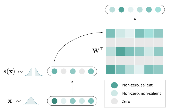
The paper that I was given to tackle was TEAL. It’s a pretty cool paper on how sparsifying the input tensors being sent into matmul kernels could reduce matmul operations by skipping over zeroed-out weights. They have a pretty nice clickbait image on their repository too that visualizes it.

I assumed that now that we have all the links, the repository, and the papers, the rest of it would be a cakewalk. But, I spent around 5 weeks iterating and understanding where I went wrong and then 3 weeks to implement it the correct way. However, this was only because I didn’t know where to look.

Where do you look? #

“Workloads”, in this context, refer to matrixes that are produced after sparsification and before multiplication with another matrix. In a single transformer block, you have two components: the Self-Attention Block and the Feed-Forward Neural Network.

The self attention block has four matrices within itself:

• Q: The Query Matrix
• K: The Key Matrix
• V: The Values Matrix
• O: The Aggregation matrix¹

The feed forward neural network has three matrices: W1, W2, W3.

The matrices in both of these blocks are used for enhancing representation of a word to be informative in contexts based on the attention scores that they get allocated. The function definitions for the blocks can be found here:

• Attention Class
• Feed Forward Neural Network

Functions that matter #

It has become a community standard to name your inference operation in a model as the “forward” operation. In gpt-fast, the authors have done the same. TEAL has too. So, we look at the code that the authors have written and understand how exactly we can modify it to extract our workloads.

Here’s the original code for the feed forward neural network:

def _new_ffn_forward(self, x: Tensor) -> Tensor:
    return self.gemv2(F.silu(self.gemv1(x, self.w1.weight, self.thresh_gate, self.sparsity_bin)) * self.gemv1(x, self.w3.weight, self.thresh_up, self.sparsity_bin), self.w2.weight, self.thresh_down, self.sparsity_bin)

class FeedForward(nn.Module):
    def __init__(self, config: ModelArgs) -> None:
        super().__init__()
        self.w1 = nn.Linear(config.dim, config.intermediate_size, bias=False)
        self.w3 = nn.Linear(config.dim, config.intermediate_size, bias=False)
        self.w2 = nn.Linear(config.intermediate_size, config.dim, bias=False)

        self.sparsify = False

    def apply_monkeypatch(self):
        self.old_forward = self.forward
        self.forward = types.MethodType(_new_ffn_forward, self)

    def forward(self, x: Tensor) -> Tensor:
        return self.w2(F.silu(self.w1(x)) * self.w3(x)) # baseline

Studying this, we see that the authors of TEAL have cleverly overloaded only the forward operation to utilize their kernel implementation through monkeypatching the forward operation to use their kernel instead.

For us, in order to retrieve the workloads that we need, we must update this monkeypatch to inject a function that can label a matrix’s layer, block, type and dump it, without affecting the inference’s output significantly.

To make this, we need to study how the authors have built up their kernel by following the trail of the self.gemv1 kernel. We do all this because there’s no easy way to drop matrices and values from within a triton kernel.

The GEMV kernel #

The GEMV kernel can be found by navigating to the entry point of the inference operation: the generate.py file, where the layers’ functions for the model are monkeypatched. This is where we find the allocation of the kernel variable, as well as the sparsification thresholds for the input tensor during pruning in the kernel.

Delving deeper, we reach the SparseGEMV kernel class, which spins up the grid for the triton kernel. This is where we find the input tensor pruning logic and the GEneral Matrix Vector multiplication taking place.

def splitk_sparse_gemv_kernel(...):
    start_n = tl.program_id(0)
    start_m = tl.program_id(1)
    # now compute the block that each program will go through
    # rn (resp. rm) denotes a range of indices for rows (resp. col) of A

    rn = start_n * BLOCK_N + tl.arange(0, BLOCK_N)
    rm = start_m * BLOCK_M + tl.arange(0, BLOCK_M)

    A_ptr = A + (rm[:, None] * N + rn[None, :])
    X_ptr = X + rm
    Y_ptr = Y + rn

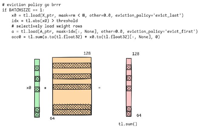
    # eviction policy go brrr
    if BATCHSIZE == 1:
        x0 = tl.load(X_ptr, mask=rm < M, other=0.0, eviction_policy='evict_last') # reuse x across threadblocks
        idx = tl.abs(x0) > threshold
        # selectively load weight rows
        a = tl.load(A_ptr, mask=idx[:, None], other=0.0, eviction_policy='evict_first') # only load weights once per threadblock
        acc0 = tl.sum(a.to(tl.float32) * x0.to(tl.float32)[:, None], 0)

    # rematerialize rm and rn to save registers
    rn = start_n * BLOCK_N + tl.arange(0, BLOCK_N)

    tl.atomic_add(Y_ptr, acc0, mask=rn < N)

Triton is a bit weird, but I’ll try to explain what’s happening here:

1. The start_n variable moves through columns while the start_m moves through rows.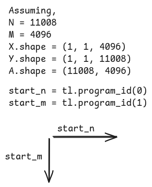

   

2. rn and rm indicate the range until which the memory space in the grid is allocated for this kernel.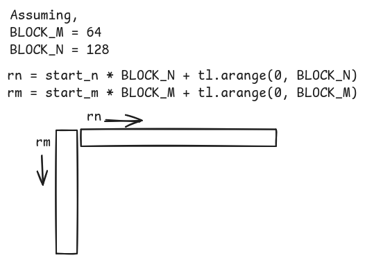

   

3. x0 loads in the values uptil the rm range.
4. The idx variable contains the values in the x0 input tensor that satisfies the threshold requirement.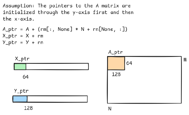

   

5. a is the result of pruning the weight matrix A post value evictions.
6. The weight matrix is multiplied with the input tensor and summed up as a matrix-vector operation.

   

7. The atomic_add operation loads in the result of this product into the output tensor.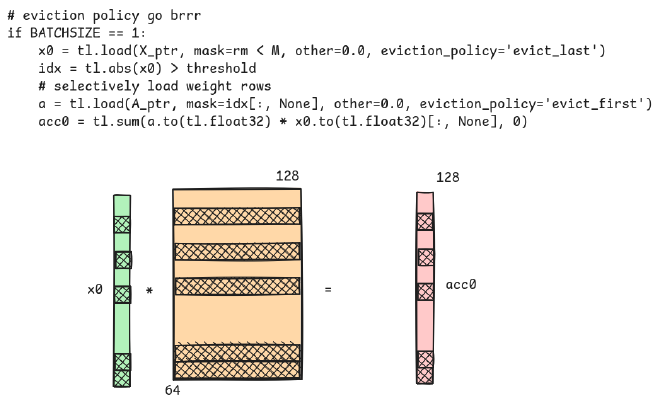

   

The simulation #

Now that we have an understanding of how the kernel works underneath the hood, we can create a function that simulates the triton kernel to dump matrices. That’s where the simulate_splitk_kernel function comes in.

def simulate_splitk(X, A, threshold, uuid):
    """Simulates the splitk gemv1 kernel"""

    N, Z = A.shape
    beam_width, seq_len, _ = X.shape

    Y = torch.empty(beam_width, seq_len, N,
                    device=X.device, dtype=torch.float16)
    mask = (X.abs() > threshold).float()
    masked = (X * mask).to(dtype=torch.float16)
    if seq_len == 1:
        for i in range(mask.shape[1]):
            input_tensor_c = masked.detach().clone().requires_grad_(False)
            torch.save(input_tensor_c, f"{uuid}.pt")
            masked_A = A * masked[0, i]
            # tensor_no_grad = masked_A.detach().clone().requires_grad_(False)
            # torch.save(tensor_no_grad, f"{uuid}.pt", _use_new_zipfile_serialization=True)
            Y[0, i] = masked_A.T.sum(axis=0)
    else:
        for i in range(mask.shape[1]):
            masked_A = A * X[0, i]
            Y[0, i] = masked_A.T.sum(axis=0)

    return Y

If we insert the necessary threshold and a UUID populated with the layer and matrix name, like in here and here, we dump the matrices with the right name.

Running it #

We’ve reached the end!

That’s pretty much how you’d manipulate the TEAL’s gpt-fast codebase to retrieve your matrix workloads. Running the actual code needs you to get rid of the compile flag because triton will attempt to compile for optimization and your dumping code is no longer going to work as easily.

For detailed steps on how you can load in thresholds and track matrices, check out this PR and go through the README for more.